
Training-Free Transformer Merging via
Sequential Local Operator Alignment
TL;DR
- Existing training-free mergers combine $\mathbf{W}_Q,\mathbf{W}_K,\mathbf{W}_V,\mathbf{W}_O$ independently — ignoring how attention operation actually operattes on inputs.
- SLOA merges the functional operators $\mathbf{W}_Q\mathbf{W}_K^{\!\top}$ and $\mathbf{W}_V\mathbf{W}_O$ directly.
- Same operator-alignment principle also handles LayerNorm and the MLP sub-blocks ($\mathbf{W}_1,\mathbf{W}_2$) — SLOA covers the whole transformer, not just attention.
- Alignment is performed sequentially on activations of the partially-merged model.
- Re-factorization lets rank act as capacity control.
- Generalizes across modalities and scales — CLIP/ViT, RoBERTa, and LoRA-adapted LLaMA-2-7B experts.
Model Merging
- $T$ task-specific models $\{\bm{\Phi}_1,\ldots,\bm{\Phi}_T\}$, each fine-tuned from the same pretrained $\bm{\Phi}_{\text{pre}}$ on its dataset $D_t$.
- Goal: aggregate them into a single multi-task model without joint retraining on $D_1\cup\cdots\cup D_T$:
- Training-free: a small unlabeled calibration set is allowed; no gradient updates.
Transformer Architecture
Multi-Head Attention (MHA). Sum of $H$ heads:
- QK circuit $\mathbf{M}_{\text{QK}}^{(j)}=\mathbf{W}_Q^{(j)}\mathbf{W}_K^{(j)\top}$ — where attention reads.
- VO circuit $\mathbf{M}_{\text{VO}}^{(j)}=\mathbf{W}_V^{(j)}\mathbf{W}_O^{(j)}$ — what is written.
- Each circuit is a $d{\times}d$ operator with a hidden rank-$d_k$ bottleneck.
MLP block. Two linear projections separated by a nonlinearity $\sigma(\cdot)$:
- SLOA aligns $\mathbf{W}_1$ on the attention output, then $\mathbf{W}_2$ on the merged post-activation $\sigma(\widehat{\mathbf{Z}}\mathbf{W}_1)$ — sequential, closed-form, same template as attention.
Motivation: Isolated merging breaks attention
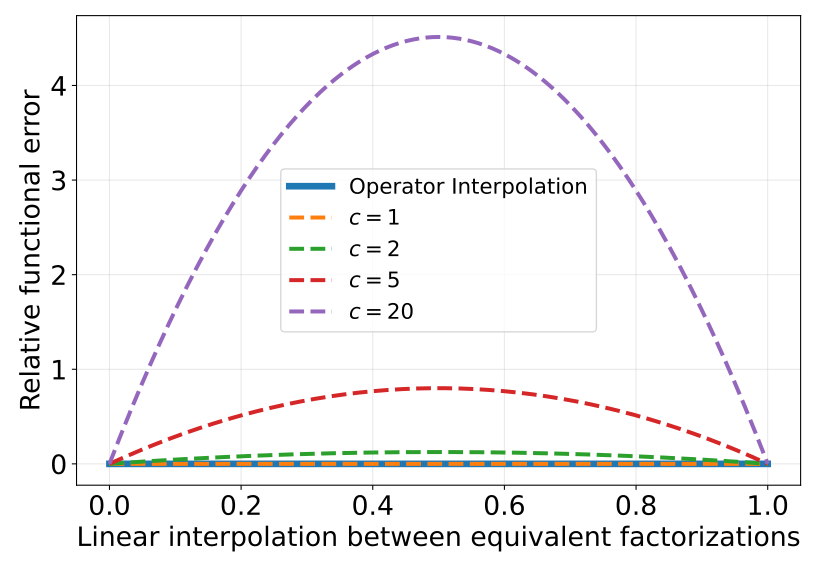
Relative functional error along linear interpolations between equivalent factorizations, grows rapidly with the scalar $c$.
- Functional unit. Attention scores depend only on the product $\mathbf{M}_{\mathrm{QK}}=\mathbf{W}_Q\mathbf{W}_K^{\!\top}$ — not on $\mathbf{W}_Q,\mathbf{W}_K$ separately.
- Hidden ambiguity. Any invertible $\mathbf{R}$ gives a different
factorization with the same function:
$$\bigl(\mathbf{W}_Q\mathbf{R}\bigr)\bigl(\mathbf{W}_K\mathbf{R}^{-\top}\bigr)^{\!\top} \;=\;\mathbf{W}_Q\mathbf{W}_K^{\!\top}.$$
- Independent averaging fails. Averaging the two parameterizations
element-wise gives
$\bar{\mathbf{W}}_Q=\tfrac{1}{2}\mathbf{W}_Q(\mathbf{I}+\mathbf{R})$,
$\bar{\mathbf{W}}_K=\tfrac{1}{2}\mathbf{W}_K(\mathbf{I}+\mathbf{R}^{-\top})$, so
$$\bar{\mathbf{M}}_{\mathrm{QK}}=\bar{\mathbf{W}}_Q\bar{\mathbf{W}}_K^{\!\top} =\tfrac{1}{4}\mathbf{W}_Q(\mathbf{I}+\mathbf{R})(\mathbf{I}+\mathbf{R}^{-1})\mathbf{W}_K^{\!\top} \;\neq\;\mathbf{W}_Q\mathbf{W}_K^{\!\top}.$$
- Unbounded blow-up. Scalar case $\mathbf{R}=c\mathbf{I}$:
$$\bar{\mathbf{M}}_{\mathrm{QK}}=\dfrac{(1+c)(1+c^{-1})}{4}\,\mathbf{M}_{\mathrm{QK}} \;\;\xrightarrow[c\to\infty]{}\;\;\infty.$$Equality holds only at $c=1$; error grows without bound otherwise.
- Consequence. Two task models that are functionally identical at the QK level can produce arbitrarily different merged attention scores under isolated weight averaging.
Key idea
- Merge at the level of local functional operators, not raw weight tensors.
- Each component's behavior is linear in its operator $\bm{\theta}$ — closed-form least squares.
- Apply alignment sequentially: each merge corrects accumulated upstream error.
- Factorize the merged operator back; the chosen rank controls multi-task capacity.
Method: Sequential Local Operator Alignment
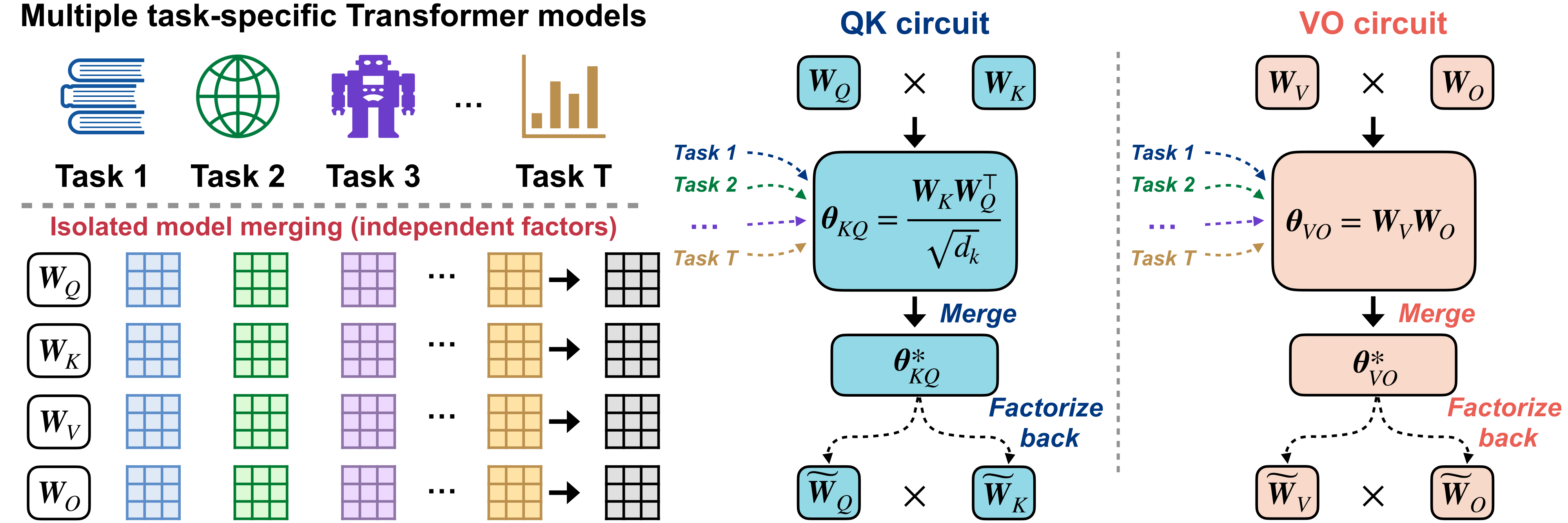
SLOA aligns the effective local operators (QK, VO, MLP, LayerNorm), merges them sequentially under partially-merged activations, then factorizes each operator back into transformer-compatible weights.
Unified alignment objective
Local operators & data-aware metrics
| Component | Local operator $\bm{\theta}$ | Behavior map $\mathcal{A}(\mathbf{Z};\bm{\theta})$ | Metric |
|---|---|---|---|
| LayerNorm | $(\bm{\gamma},\bm{\beta})$ | $\nu(\mathbf{X})\,\mathrm{diag}(\bm{\gamma})+\mathbf{1}\bm{\beta}^{\!\top}$ | $\mathrm{Cov}(\nu(\chi))$ |
| Linear map | $\mathbf{W}$ | $\mathbf{X}\mathbf{W}$ | $\bm{\Lambda}$ |
| QK component | $\dfrac{1}{\sqrt{d_k}}\mathbf{W}_Q\mathbf{W}_K^{\!\top}$ | $\mathbf{X}\bm{\theta}\mathbf{X}^{\!\top}$ | $\bm{\Lambda}\otimes\bm{\Lambda}$ |
| VO component | $\mathbf{W}_V\mathbf{W}_O$ | $\mathbf{A}\mathbf{X}\bm{\theta}$ | $\bm{\Lambda}$ |
$\nu(\mathbf{X})$ is the LayerNorm-normalized input; $\mathbf{A}$ is the attention matrix; $\bm{\Lambda}=\alpha\,\mathrm{diag}\bigl(\mathrm{Cov}(\mathbf{X})\bigr)+\epsilon\mathbf{I}$.
- Activation term matches local input–output behavior on calibration data.
- Geometry term is a Mahalanobis distance: penalizes deviation along directions the calibration activations actually use.
- For fixed activations the objective is quadratic in $\bm{\theta}$ — closed-form regularized least squares per component.
- Sequential: downstream operators are aligned on activations from the partially merged model $\widehat{\mathbf{Z}}$.
Rank as capacity control
After merging the QK / VO operator in $\mathbb{R}^{d\times d}$, SVD the operator $\bar{\bm{\theta}}=\mathbf{U}\bm{\Sigma}\mathbf{V}^{\!\top}$ and factorize at chosen rank $r_j$.
QK circuit (with denominator $c_j=\sqrt{r_j}$):
VO circuit:
- $r_j = d_k$ preserves the original head width.
- $r_j > d_k$ retains additional task-specific singular directions.
- The sum of task heads can span a larger subspace than any single rank-$d_k$ head — expansion avoids unnecessary truncation.
SLOA in 4 steps
- Collect activations $\{\mathbf{Z}_{t,i}\}$ for each operator from a small calibration set.
- Order operators topologically $o_1\!\prec\!\cdots\!\prec\!o_M$ (LayerNorm $\to$ QK $\to$ VO $\to$ MLP).
- For each $o_m$: forward through the partially-merged model to get $\widehat{\mathbf{Z}}_{t,i}$, then solve closed-form regularized LS.
- Factorize QK/VO via SVD at chosen rank $r_j$ and write back transformer-compatible weights.
No gradients, no labels — one deterministic pass through the operator graph.
Vision: Merging ViT-B/32 (CLIP fine-tunes)
Table 1. Average classification accuracy (%) of the merged model under three increasingly difficult settings: 8, 14, and 20 task-specific ViT-B/32 models. Higher is better; training-free methods use 256 calibration examples per task. For SLOA, $r$ is the retained QK/VO factorization rank ($r{=}64$ matches the original head dimension).
| Method | Samples | Avg. Accuracy (%) $\uparrow$ | |||
|---|---|---|---|---|---|
| 8 tasks | 14 tasks | 20 tasks | |||
| Fine-tuned | – | 90.39 | 89.26 | 89.78 | |
| Data-Free | Weight Averaging | – | 66.29 | 65.37 | 61.08 |
| Task Arithmetic | – | 69.49 | 66.47 | 60.60 | |
| TIES-Merging | – | 71.70 | 67.58 | 62.76 | |
| TSV-M | – | 83.04 | 79.11 | 73.66 | |
| Iso-C | – | 82.64 | 77.94 | 71.16 | |
| Iso-CTS | – | 82.87 | 79.24 | 73.41 | |
| Training-Free | Fisher Merging | 256 | 69.12 | 66.26 | 61.74 |
| RegMean | 256 | 82.63 | 77.93 | 72.20 | |
| RegMean++ | 256 | 84.37 | 80.06 | 74.51 | |
| SLOA ($r{=}64$) | 256 | 84.89 | 81.94 | 80.06 | |
| SLOA ($r{=}128$) | 256 | 85.50 | 82.61 | 81.03 | |
- Even at the original rank, SLOA is the best method on all three benchmarks; the gap widens with more tasks.
- Margin over RegMean++ at $r{=}64$: +0.6 (8t), +1.9 (14t), +5.5 pts (20t).
- Rank expansion $r{=}64{\to}128$ consistently helps — the merged operator's spectrum spans a larger subspace than any single head.
NLU: Merging RoBERTa on 7 GLUE tasks
Table 2. Per-task and average Metric of the merged RoBERTa model on seven GLUE tasks (CoLA, SST-2, MRPC, QQP, MNLI, QNLI, RTE). Higher is better; training-free methods use 256 calibration examples per task. SLOA ($r{=}64$) preserves the original head rank; SLOA ($r{=}128$) expands the QK/VO factorization rank.
| Method | Samples | Metric $\uparrow$ | ||||||||
|---|---|---|---|---|---|---|---|---|---|---|
| CoLA | SST-2 | MRPC | QQP | MNLI | QNLI | RTE | Avg | |||
| Individual | – | 0.6018 | 0.9404 | 0.8922 | 0.9141 | 0.8720 | 0.9271 | 0.7906 | 0.8483 | |
| Data-Free | Weight Averaging | – | 0.1808 | 0.8188 | 0.8116 | 0.7381 | 0.4383 | 0.7106 | 0.6173 | 0.6165 |
| Task Arithmetic | – | 0.2909 | 0.8463 | 0.8188 | 0.7869 | 0.5591 | 0.7584 | 0.6462 | 0.6724 | |
| TIES-Merging | – | 0.1951 | 0.8429 | 0.8333 | 0.8351 | 0.6501 | 0.7309 | 0.4260 | 0.6448 | |
| TSV-M | – | 0.3477 | 0.8739 | 0.8446 | 0.8286 | 0.6163 | 0.8124 | 0.6606 | 0.7120 | |
| Iso-C | – | 0.2639 | 0.8601 | 0.8130 | 0.8211 | 0.7303 | 0.7882 | 0.7040 | 0.7115 | |
| Iso-CTS | – | 0.4136 | 0.7798 | 0.6385 | 0.6500 | 0.5277 | 0.6590 | 0.6534 | 0.6174 | |
| Training-Free | Fisher Merging | 256 | 0.1126 | 0.8719 | 0.7419 | 0.7808 | 0.4227 | 0.5311 | 0.5150 | 0.5680 |
| RegMean | 256 | 0.2797 | 0.8933 | 0.8069 | 0.7915 | 0.7251 | 0.8336 | 0.6161 | 0.7066 | |
| RegMean++ | 256 | 0.2433 | 0.9170 | 0.7740 | 0.8099 | 0.7543 | 0.8299 | 0.6691 | 0.7139 | |
| SLOA ($r{=}64$) | 256 | 0.5608 | 0.9232 | 0.8814 | 0.8152 | 0.7678 | 0.8755 | 0.7100 | 0.7906 | |
| SLOA ($r{=}128$) | 256 | 0.5721 | 0.9239 | 0.8810 | 0.8166 | 0.7753 | 0.8824 | 0.7341 | 0.7979 | |
bold = best in column; underline = second best. SLOA is best on 6/7 tasks; +8.4 avg. pts over the strongest baseline at $r{=}128$.
Ablations
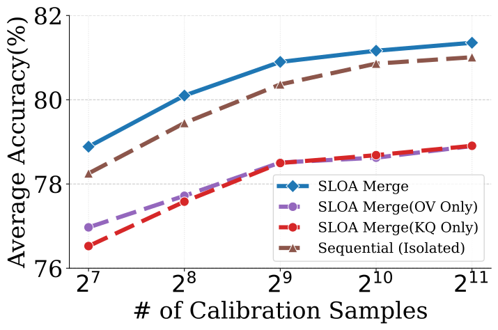
Component ablation (20 tasks)
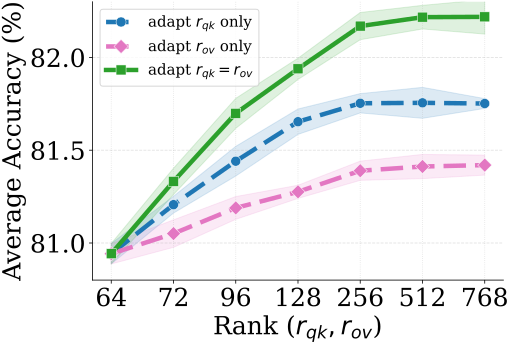
Decoupling QK and OV ranks
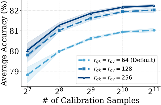
Scaling with calibration & rank (ViT-B/32, 20 tasks)
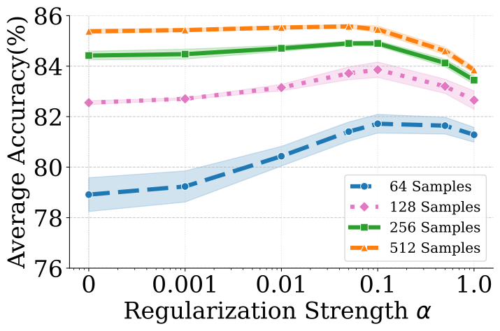
Sensitivity to regularization $\alpha$
- Sequential alignment alone is already strong.
- QK and OV must be merged jointly — isolating one hurts.
- Jointly expanding QK and OV ranks gives the best, most sustained gains.
- Optimal $\alpha$ decreases as more calibration data is available.
Task-wise comparison: SLOA vs. data-free and training-free baselines
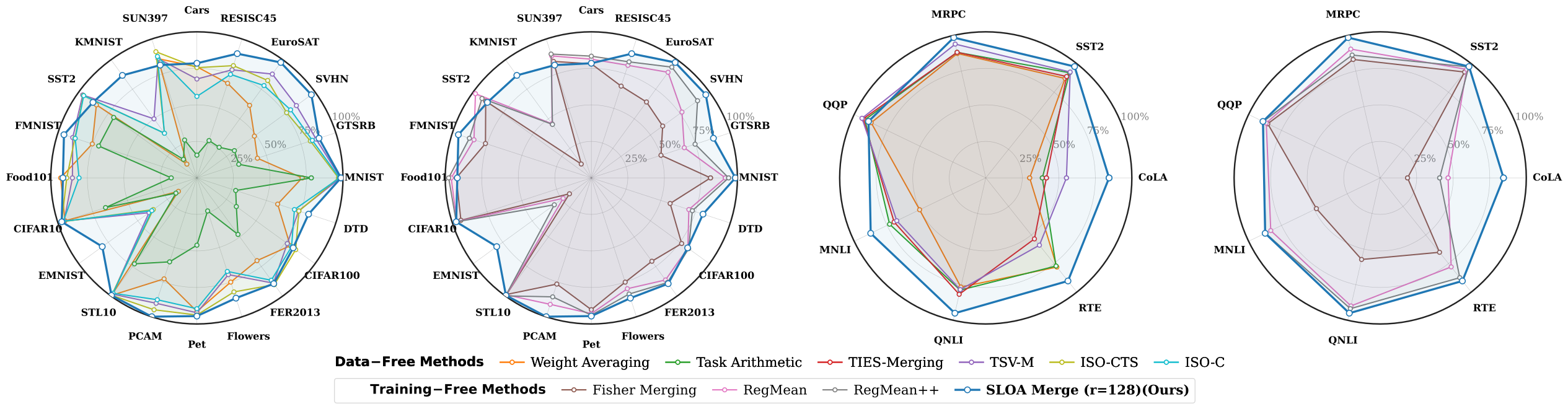
From left to right: ViT-B/32 on 20 vision tasks vs. data-free / vs. training-free baselines; RoBERTa on 7 GLUE tasks vs. data-free / vs. training-free baselines. SLOA ($r{=}128$) consistently outperforms both data-free and training-free baselines.
Conclusions & Limitations
Take-aways
- Treat $\mathbf{W}_Q\mathbf{W}_K^{\!\top}$ and $\mathbf{W}_V\mathbf{W}_O$ as the units to merge — not the raw matrices.
- Sequential, data-aware alignment removes parameterization ambiguity and curbs cross-layer error accumulation.
- Rank expansion grows multi-task capacity without training.
- Generalizes from CLIP and RoBERTa to LoRA-adapted LLaMA-2-7B experts (SLOA-VO: 49.19 avg. vs. 46.46 for RegMean++).
Limitations
- Needs calibration data — more than purely data-free baselines require.
- Higher offline merging cost: 182 s vs. 84–115 s for RegMean/RegMean++ on 20-task ViT-B/16 — strictly one-time, no backprop.
- Rank expansion increases inference cost: per-head $O(L^2 r_j)$ when $r_j>d_k$; trade-off between capacity and latency.
Future work
- Reduce calibration / merging cost and automatically select per-head ranks under deployment budgets.
- Compose the QK operator under rotary position embeddings (currently VO-only for LLaMA).
- Extend operator-level merging to encoder-decoder transformers.

github.com/akansh12/SLOA-Merge

linkedin.com/in/akansh-maurya