Coding the Genetic Algorithm using MATLAB
Guided by Dr. Nitin Anand Srivastava
(Institute of Engineering and Technology, Lucknow)
Abstract
In computer science and operations research, a genetic algorithm (GA) is a metaheuristic inspired by the process of natural selection that belongs to the larger class of evolutionary algorithms (EA). Genetic algorithms are commonly used to generate high-quality solutions to optimization and search problems by relying on bio-inspired operators such as mutation, crossover, and selection. John Holland introduced genetic algorithms in 1960 based on the concept of Darwin’s theory of evolution; afterward, his student David E. Goldberg extended GA in 1989.
Introduction
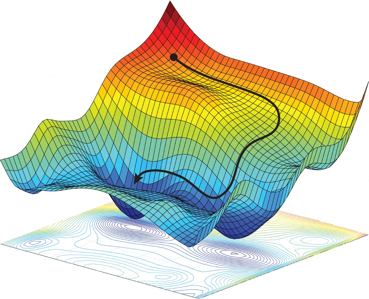
An optimization is an important tool in making decisions and in analyzing
physical systems. In mathematical terms, an optimization problem is a problem
of finding the best solution from among the set of all feasible solutions. Genetic Algorithms (GA) are the
heuristic search and optimization techniques that mimic the process of natural evolution.
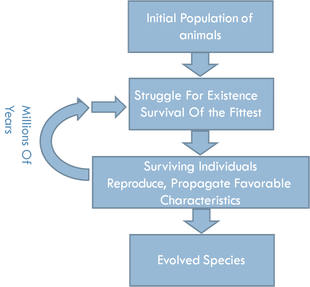
An Example: Giraffes evolving long necks.
- Giraffes with slightly longer necks could feed on leaves of higher branches when all lower ones had been eaten off.
- They had a better chance of survival.
- Favorable characteristics propagated through generations of giraffes.
- Now, evolved species have long necks.
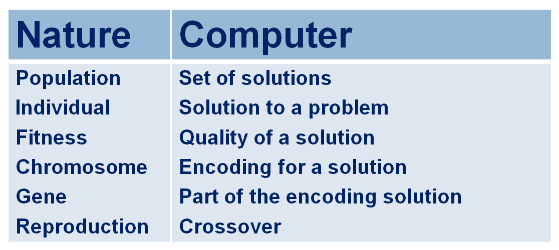
GA Operators and Parameters
- Selection
- Crossover
- Mutation
- Elitism
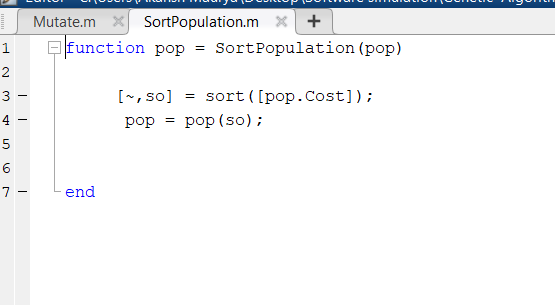
Selection:
A fitness function value quantifies the optimality of a solution. The value is used to rank a particular solution against all the other solutions. A fitness value is assigned to each solution depending on how close it is actually to the optimal solution of the problem.
Crossover:
The crossover operator is used to create new solutions from the existing solutions available in the mating pool after applying the selection operator. This operator exchanges the gene information between the solutions in the mating pool. The most popular crossover selects any two solutions strings randomly from the mating pool and some portion of the strings is exchanged between the strings.
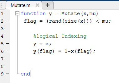
Mutation:
The mutation is the occasional introduction of new features into the solution strings of the population pool to maintain diversity in the population. Though crossover has the main responsibility to search for the optimal solution, the mutation is also used for this purpose. The mutation operator changes a 1 to 0 or vice versa, with a mutation probability of 0.1 or near. The mutation probability is generally kept low for steady convergence. A high value of mutation probability would search here and there like a random search technique.
Elitism:
Elitism is the preservation of the few best solutions for the population pool.
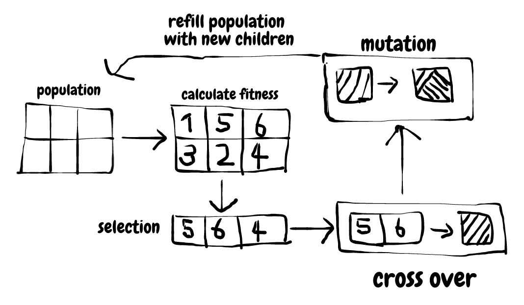
Coding the Genetic Algorithm
General method:
    function ga()
{
Initialize population;
Calculate the fitness function;
While(fitness value != termination criteria)
{
Selection;
Crossover; Mutation;
Calculate the fitness function;
}
}
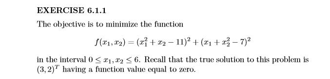
Problem Statement:
Solution: https://github.com/akansh12/Genetic-Algorithim-using-MATLAB
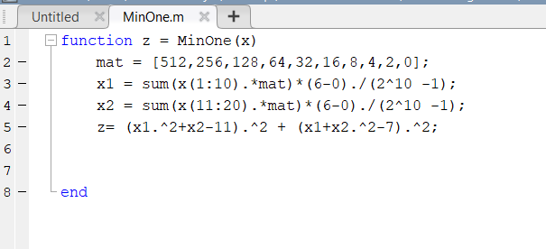
Problem Definition:
Note: Selection is done in the main Script.
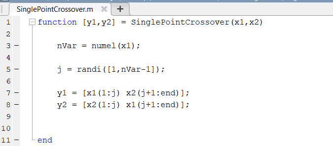
Crossover:
Mutation:
Elitism:
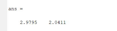
Results:
Number of genes: 10
Number of iteration: 100
Crossover Probability: 0.8
Mutation Probability: 0.1
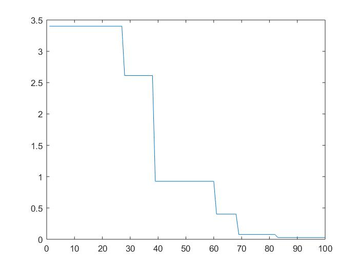
X1 and X2 respectively shown below: